Reviewing the basics of matrices for differential equations

A basic review of matrices for differential equations
We’ll learn much more about matrices in Linear Algebra. For now, we just need a brief introduction to matrices (for some, this may be a review from Precalculus), since we’ll be using them extensively to solve systems of differential equations.

Hi! I'm krista.
I create online courses to help you rock your math class. Read more.
Dimensions, systems, and multiplication
The first thing we’ll say is that an ???n\times m??? matrix is an array of entries with ???n??? rows and ???m??? columns. These are examples of square ???2\times2??? and ???3\times3??? matrices:

We can use matrices to represent a system of equations. For instance, given the system,
???3x_1-4x_2=2???
???x_1+5x_2=-1???
we can rewrite it using one matrix equation as

A single column matrix can also be thought of as a vector, so this matrix equation has the coefficient matrix multiplied by the vector ???\vec{x}=(x_1,x_2)???, set equal to the vector ???\vec{b}=(2,-1)???. When we multiply two matrices, as we’re doing on the left side of this equation, we always multiply the row(s) in the first matrix by the column(s) in the second matrix. In other words, working our way across the first row of this matrix equation gives us back the first equation from the system,
???(3)(x_1)+(-4)(x_2)=2???
???3x_1-4x_2=2???
and working our way across the second row of this matrix equation gives us back the second equation from the system.
???(1)(x_1)+(5)(x_2)=-1???
???x_1+5x_2=-1???
We just looked at multiplying the ???2\times2??? matrix by the ???2\times1??? matrix/vector, but it’s also important to say that we can multiply any matrix by a scalar. To do so, we just distribute the scalar across every entry in the matrix.

And to add or subtract matrices, we simply add or subtract corresponding entries.

Determinants
We’ll also need to know how to calculate the determinant for a matrix. For a ???2\times2??? matrix, the determinant is given by

For a ???3\times3??? matrix, the determinant is given by

Take special notice of the negative sign in front of ???b???. When we break down the determinant, we add the ???a??? and ???c??? terms, but subtract the ???b??? term. Then the determinant simplifies as

Eigenvalues and Eigenvectors
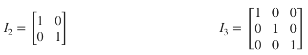
The identity matrix is a square matrix with all ???0??? entries, except for the main diagonal, running from the top left to lower right, which is filled with ???1???s. Here are the ???2\times2??? and ???3\times3??? identity matrices:
Later we’ll need to be able to find the Eigenvalues and Eigenvectors of a matrix. The Eigenvalues of the matrix are the values of ???\lambda??? that satisfy ???|A-\lambda I|=0???. For instance, these are the steps we’d take to find the Eigenvalues of the ???2\times2??? matrix we used earlier:

Take the determinant,

then solve the characteristic equation ???\lambda^2-8\lambda+19=0??? for the Eigenvalues. We’ll get the Eigenvector associated with each Eigenvalue by putting the matrix ???A-\lambda I??? into row-echelon form using Gauss-Jordan elimination, and then solving the system given by the simplified matrix.
Gauss-Jordan elimination algorithm
One way to think about the goal of this algorithm (a specific set of steps that can be repeated over and over again) is that we’re trying to rewrite the matrix so that it’s as similar as possible to the identity matrix.
In other words, we’re trying to change all the entries along the main diagonal to ???1???, and all the other entries to ???0???. We won’t always be able to get to the identity matrix exactly, but we’ll try to get as close as possible.
If the first entry in the first row is ???0???, swap it with another row that has a non-zero entry in its first column. Otherwise, move to step 2.
Multiply through the first row by a scalar to make the leading entry equal to ???1???.
Add scaled multiples of the first row to every other row in the matrix until every entry in the first column, other than the leading ???1??? in the first row, is a ???0???.
Go back to step 1 and repeat the process until the matrix is in reduced row-echelon form.
For instance, to put our ???2\times2??? matrix into row-echelon form, we’ll divide through the first row by ???3??? in order to change the first entry from ???3??? to ???1???.

Then to change the ???1??? in the second row into a ???0???, we’ll subtract the first row from the second, and use the result to replace the second row.

Then to change the ???19/3??? to a ???1???, we’ll multiply through the second row by ???3/19???.

Then to zero out the ???-4/3???, we’ll add ???4/3??? of the second row to the first row.

In this case, the matrix does reduce down to the identity matrix. As we mentioned though, this won’t always be the case.