Correlation coefficients and the residual
Defining the correlation coefficient
In the last section we talked about the regression line, and how it was the line that best represented the data in a scatterplot.
In this section, we’re going to get technical about different measurements related to the regression line.

Hi! I'm krista.
I create online courses to help you rock your math class. Read more.
Correlation coefficient, r
The correlation coefficient, denoted with ???r???, tells us how strong the relationship is between ???x??? and ???y???. It’s given by
???r=\frac{1}{n-1}\sum\left(\frac{x_i-\bar{x}}{s_x}\right)\left(\frac{y_i-\bar{y}}{s_y}\right)???
Notice that in this formula for correlation coefficient, we have the values ???(x_i-\bar{x})/s_x??? and ???(y_i-\bar{y})/s_y???, where ???s_x??? and ???s_y??? are the standard deviations with respect to ???x??? and ???y???, and ???\bar{x}??? and ???\bar{y}??? are the means of ???x??? and ???y???. Therefore ???(x_i-\bar{x})/s_x??? and ???(y_i-\bar{y})/s_y??? are the ???z???-scores for ???x??? and ???y???, which means we could also write the correlation coefficient as
???r=\frac{1}{n-1}\sum(z_{x_i})(z_{y_i})???
The value of the correlation coefficient will always fall within the interval ???[-1,1]???. If ???r=-1???, it indicates that a regression line with a negative slope will perfectly describe the data. If ???r=1???, it indicates that a regression line with a positive slope will perfectly describe the data. If ???r=0???, then we can say that a line doesn’t describe the data well at all. In other words, the data may just be a big blob (no association), or sharply parabolic. In other words, the relationship is nonlinear.
Don’t confuse a value of ???r=-1??? with a slope of ???-1???. A correlation coefficient of ???r=-1??? does not mean the slope of the regression line is ???-1???. It simply means that some line with a negative slope (we’re not sure what the slope is, we just know it’s negative) perfectly describes the data.
“Perfectly describes the data” means that all of the data points lie exactly on the regression line. In other words, the closer ???r??? is to ???-1??? or ???1??? (or the further it is away from ???0???, in either direction), the stronger the linear relationship. If ???r??? is close to ???0???, it means the data shows a weaker linear relationship.
Understanding correlation coefficients and the residual

Take the course
Want to learn more about Probability & Statistics? I have a step-by-step course for that. :)
How to find the correlation coefficient
Example
Using the data set from the last section, find the correlation coefficient.
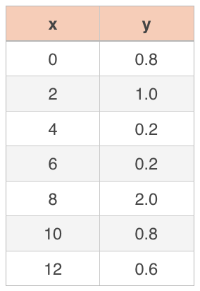
First, we need to find both means, ???\bar x??? and ???\bar y???,
???\bar x=\frac{0+2+4+6+8+10+12}{7}=\frac{42}{7}=6???
???\bar y=\frac{0.8+1.0+0.2+0.2+2.0+0.8+0.6}{7}=\frac{5.6}{7}=0.8???
and both standard deviations ???s_x??? and ???s_y???.
???s_x=\sqrt{\frac{\sum_{i=1}^7(x_i-\bar x)^2}{7}}=\sqrt{\frac{36+16+4+0+4+16+36}{7}}=\sqrt{16}=4???
???s_y=\sqrt{\frac{\sum_{i=1}^7(y_i-\bar y)^2}{7}}=\sqrt{\frac{0+0.04+0.36+0.36+1.44+0+0.04}{7}}\approx0.5657???
Then if we plug these values for ???\bar{x}???, ???\bar{y}???, ???s_x???, and ???s_y???, plus the points from the data set, into the formula for the correlation coefficient, we get
???r=\frac{1}{n-1}\sum\left(\frac{x_i-\bar{x}}{s_x}\right)\left(\frac{y_i-\bar{y}}{s_y}\right)???
???r=\frac{1}{7-1}\Bigg[\left(\frac{0-6}{4}\right)\left(\frac{0.8-0.8}{0.5657}\right)+\left(\frac{2-6}{4}\right)\left(\frac{1.0-0.8}{0.5657}\right)???
???+\left(\frac{4-6}{4}\right)\left(\frac{0.2-0.8}{0.5657}\right)+\left(\frac{6-6}{4}\right)\left(\frac{0.2-0.8}{0.5657}\right)+\left(\frac{8-6}{4}\right)\left(\frac{2.0-0.8}{0.5657}\right)???
???+\left(\frac{10-6}{4}\right)\left(\frac{0.8-0.8}{0.5657}\right)+\left(\frac{12-6}{4}\right)\left(\frac{0.6-0.8}{0.5657}\right)\Bigg]???
???r=\frac{1}{6}\Bigg[-\frac32\left(\frac{0}{0.5657}\right)-1\left(\frac{0.2}{0.5657}\right)???
???-\frac12\left(\frac{-0.6}{0.5657}\right)+0\left(\frac{-0.6}{0.5657}\right)+\frac12\left(\frac{1.2}{0.5657}\right)???
???+1\left(\frac{0}{0.5657}\right)+\frac32\left(\frac{-0.2}{0.5657}\right)\Bigg]???
???r=\frac{1}{6}\left[-\frac{0.2}{0.5657}+\frac12\left(\frac{0.6}{0.5657}\right)+\frac12\left(\frac{1.2}{0.5657}\right)-\frac32\left(\frac{0.2}{0.5657}\right)\right]???
???r\approx\frac{1}{6}(-0.3535+0.5303+1.0606-0.5303)???
???r\approx0.1179???
This positive correlation coefficient tells us that the regression line will have a positive slope. The fact that the positive value is much closer to ???0??? than it is to ???1??? tells us that the data is very loosely correlated, or that it has a weak linear relationship. And if we look at a scatterplot of the data that includes the regression line, we can see how this is true.
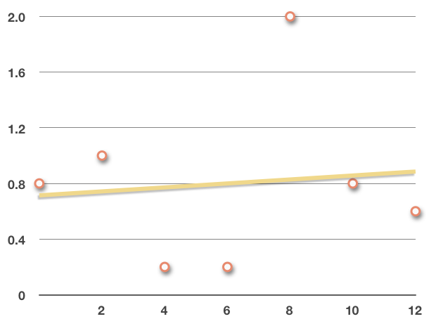
In this graph, the regression line has a positive slope, but the data is scattered far from the regression line, with several outliers, such that the relationship is weak.

“Perfectly describes the data” means that all of the data points lie exactly on the regression line.
In general, the data set has a
strong negative correlation when ???-1<r<-0.7???
moderate negative correlation when ???-0.7<r<-0.3???
weak negative correlation when ???-0.3<r<0???
weak positive correlation when ???0<r<0.3???
moderate positive correlation when ???0.3<r<0.7???
strong positive correlation when ???0.7<r<1???
Residual, e
The residual for any data point is the difference between the actual value of the data point and the predicted value of the same data point that we would have gotten from the regression line.
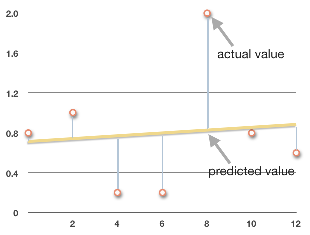
The blue lines in the chart represent the residual for each point. Notice that the absolute value of the residual is the distance from the predicted value on the line to the actual value of the point. The point ???(8,2)??? will have a large residual because it’s far from the regression line, and the point ???(10,0.8)??? will have a small residual because it’s close to the regression line.
If the data point is below the line, the residual will be negative; if the data point is above the line, the residual will be positive. In other words, to find the residual, we use the formula
???\text{residual}=\text{actual}-\text{predicted}???
The residual then is the vertical distance between the actual data point and the predicted value. Many times we use the variable ???e??? to represent the residual (because we also call the residual the error), and we already know that we represent the regression line with ???\hat{y}???, which means we can also state the residual formula as
???e=y-\hat{y}???
Now that we know about the residual, we can characterize the regression line in a slightly different way than we have so far.
For any regression line, the sum of the residuals is always ???0???,
???\sum e=0???
and the mean of the residuals is also always ???0???.
???\bar{e}=0???
If we have the equation of the regression line, we can do a simple linear regression analysis by creating a chart that includes the actual values, the predicted values, and the residuals. We do this by charting the given ???x??? and ???y??? values, then we can evaluate the regression line at each ???x???-value to get the predicted value ???\hat{y}??? (“y-hat”), and find the difference between ???y??? and ???\hat{y}??? to get the residual, ???e???.
If we use the same data set we’ve been working with, then the equation of the regression line is
???y=0.0143x+0.7143???
and we can do the simple linear regression analysis by filling in the chart.

Notice how, if you compare the chart to the scatterplot with the regression line, the negative residuals correspond to points below the regression line, and the positive residuals correspond to points above the regression line.
If we make a new scatterplot, with the independent variable along the horizontal axis, and the residuals along the vertical axis, notice what happens to the regression line.
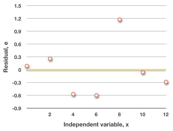
This should make sense, since we said that the sum and mean of the residuals are both always ???0???. Whenever this graph produces a random pattern of points that are spread out below ???0??? and above ???0???, that tells you that a linear regression model will be a good fit for the data.
On the other hand, if the pattern of points in this plot is non-random, for instance, if it follows a u-shaped parabolic pattern, then a linear regression model will not be a good fit for the data.
Minimizing residuals
To find the very best-fitting line that shows the trend in the data (the regression line), it makes sense that we want to minimize all the residual values, because doing so would minimize all the distances, as a group, of each data point from the line-of-best-fit.
In order to minimize the residual, which would mean to find the equation of the very best fitting line, we actually want to minimize
???\sum (r_n)^2???
where ???r_n??? is the residual for each of the given data points.
We square the residuals so that the positive and negative values of the residuals do not equal a value close to ???0??? when they’re summed together, which can happen in some data sets when you have residuals evenly spaced both above and below the line of best fit. Squaring them takes out the negative values and keeps them from canceling each other out so that all the residuals can be minimized.

This process of trying to minimize residuals by minimizing the squares of the residuals, is where we get the names least-squares-line, line of least squares, and least-squares regression. We’re trying to minimize the area of the squares.