Coefficient of determination and root-mean-square error (RMSE)

Finding the coefficient of determination
At the end of the last section, we said that, in order to find the equation of the line-of-best-fit, we actually want to minimize
???\sum (r_n)^2???
where ???r_n??? is the residual for each data point.

Hi! I'm krista.
I create online courses to help you rock your math class. Read more.
Coefficient of determination
If ???r_n??? is the residual, the next thing we want to talk about is ???r^2???, the coefficient of determination. But let’s take a step back for a moment.
We’ve been talking about finding the regression line that best approximates the trend in the data. But we could have simply found the average of all the ???y???-values in the set and then drawn a horizontal line through the data at that point instead.
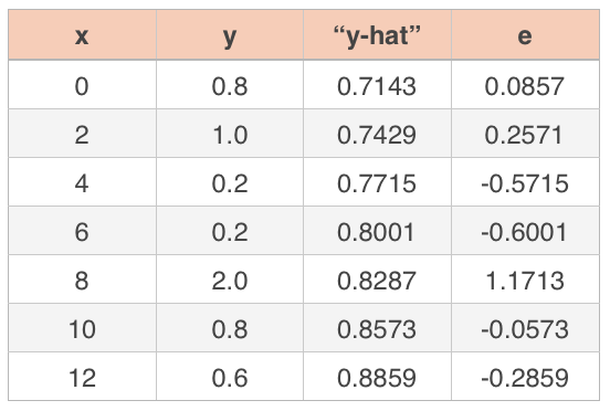
For instance, given the data set

the mean of the ???y???-values is
???\bar y=0.8???
So, instead of sketching in the regression line, we could have taken a simpler path and sketched in the horizontal line at ???\bar y=0.8???.
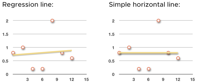
The horizontal line doesn’t fit the data as well as the regression line, but it’s much faster to find. What we want to talk about now is how much error we eliminate by using the regression line, instead of the horizontal line.
If we eliminate a large amount of error, then we know that the regression line is a much better approximation than the simpler horizontal line. But if we only eliminate a small amount of error, then we know the horizontal line was actually a pretty good trend line for the data, and that the regression line doesn’t do much better.
So how do we find the amount of error eliminated by using the regression line instead of the horizontal line? We do it with the coefficient of determination, ???r^2???, which measures the percentage of error we eliminated by using least-squares regression instead of just ???\bar{y}???.
We already know that the residual ???r??? of a data point is the distance between the point’s actual ???y???-value and its predicted ???\hat{y}???-value from the regression line.
For the horizontal line through the data, if we were to take the residual of each data point and square it, and then add up the area inside all of those actual squares, we’d get a “sum of squares” that, in a way, measures the error of just drawing the horizontal line.
If instead we find the regression line that more accurately fits the data, and then we go through the same procedure of finding the residual for each data point compared to the regression line, and take the sum of squares again, what we’ll find is that we significantly reduce the sum of squares, and therefore reduce the error. In other words, ???r^2??? tells us how well the regression line approximates the data.
For this reason, the coefficient of determination is often written as a percent, where ???100\%??? would describe a line that’s a perfect fit to the data. The higher the value of ???r^2???, the more data points the line passes through. If ???r^2??? is very small, it means the regression line doesn’t pass through many of the data points.
The coefficient of determination is the square of the correlation coefficient, which is why we use ???r??? for correlation coefficient and ???r^2??? for coefficient of determination.
Root-mean-square error
Root-mean-square error (RMSE), also called root-mean-square deviation (RMSD), you can think of as the standard deviation of the residuals.
In the same way that we talked about the standard deviation of normally distributed data, and how many data points fall within one, two, or three standard deviations from the mean, we can think about RMSE as the standard deviation of the data away from the least-squares line.
Once we find the least-squares line, and we’ve sketched that through the data, we could draw parallel lines on either side of the least-squares line that represent standard deviations away from the regression line. If the standard deviation is very large, and these lines are far from the least-squares line, it tells us that the least-squares line doesn’t fit the data very well. But if the standard deviation is very small, and these lines are close to the least-squares line, it tells us that the least-squares line does a very good job showing the trend in the data.
To find RMSE, you’ll find the residual for each data point, then square it. You’ll add up all of those square residuals, and then divide by ???n-1???, just like when we were taking sample standard deviation, instead of population standard deviation. Then you’ll take the square root of that result, and you’ll get the standard deviation of the residuals.
If we continue on with the data set we’ve been working with,
we want to start by squaring the residuals.
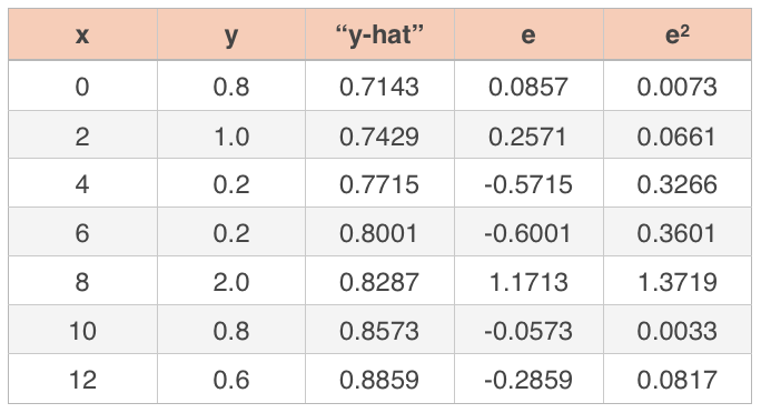
Then we sum the residuals, divide that sum by ???n-1???, and take the square root of that result. Since we have ???n=7??? data points, we get
???RMSE\approx\sqrt{\frac{0.0073+0.0661+0.3266+0.3601+1.3719+0.0033+0.0817}{7-1}}???
???RMSE\approx\sqrt{\frac{2.2170}{6}}???
???RMSE\approx0.6079???
This value is the standard deviation of the residuals, which means that, based on the normal curve from earlier in the course,

???68\%??? of the data points will fall within ???\pm0.6079??? (one standard deviation) of the regression line, that ???95\%??? of the data points will fall within ???\pm2(0.6079)??? (two standard deviations) of the regression line, and that ???99\%??? of the data points will fall within ???\pm3(0.6079)??? (three standard deviations) of the regression line.
We could roughly sketch these standard deviation boundaries into the graph.
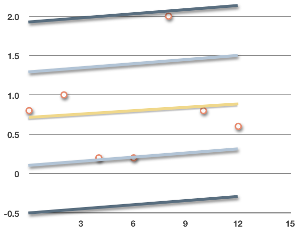
???68\%??? of the data points will fall inside the light blue lines, and ???95\%??? of the data will fall inside the dark blue lines.
The larger the RMSE (standard deviation),
the further apart these lines will be,
the more scattered the data points are, and
the weaker the correlation is in the data
The smaller the RMSE (standard deviation),
the closer together these lines will be,
the more tightly clustered the data points are, and
the stronger the correlation is in the data