Chi-square tests

Three kinds of chi-square tests
There are three kinds of ???\chi^2???-tests (chi-squared) we want to look at.
A ???\chi^2???-test for homogeneity
A ???\chi^2???-test for association/independence
???\chi^2???-test with a contingency table

Hi! I'm krista.
I create online courses to help you rock your math class. Read more.
In general, ???\chi^2???-tests let you investigate the relationship between categorical variables. For instance the ???\chi^2???-test for homogeneity is a test you can use to determine whether the probability distributions for two different groups are homogeneous. Whereas the ???\chi^2???-test for association lets you determine whether two variables are related in the same group.
We’ll cover all three of these ???\chi^2???-tests in much more detail in this section. But first, we need to remember our conditions for sampling, since we’ll often be using samples to represent populations in ???\chi^2??? problems.
Conditions for inference
Sometimes you’ll have a ???\chi^2??? problem where someone’s taking a sample of a population. When sampling occurs, in order for us to be able to use a ???\chi^2???-test, we need to be able to meet typical sampling conditions:
Random: Any sample we’re using needs to be taking randomly.
Large counts: Each expected value (more on “expected value” later) that we calculate needs to be ???5??? or greater.
Independent: We should be sampling with replacement, but if we’re not, then the sample we take shouldn’t be larger than ???10\%??? of the total population.
If any of these conditions aren’t met, we can’t use a ???\chi^2??? testing method. But assuming we can meet these three conditions, then each of these three ???\chi^2???-tests looks pretty much the same.
???\chi^2???-test for homogeneity
When we use a ???\chi^2???-test for homogeneity, we’re trying to determine whether the distributions for two variables are similar, or whether they differ from each other.
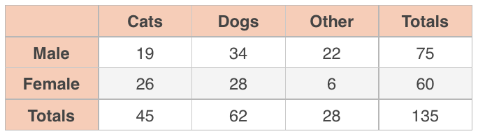
Let’s use an example. Say you take a sample of male students and a sample of female students and ask all of them whether they prefer cats, dogs, or some other animal as pets.
This is a ???\chi^2???-test for homogeneity because we’re sampling from two different groups (males and females) and comparing their probability distributions.
So in this study you have two variables, gender and pet, and you want to know whether gender affects pet preference, or if pet preference is not affected at all by gender. If pet preference isn’t affected by gender, then the distribution of pet preference for males should be the same or similar to the distribution of pet preference for females. If gender does affect pet preference, then the distributions will be different (they won’t be homogeneous).
To test this, you want to state the null hypothesis, which will be that gender doesn’t affect pet preference.
???H_0???: gender doesn’t affect pet preference
???H_a???: pet preference is affected by gender
The totals in the table margins let you determine the overall probability of being male or female in this study, regardless of pet preference, and the overall probability of preferring cats, dogs, or some other pet, regardless of gender.
If the distributions for pet preference for males and females are homogeneous, then you should be able to use these marginal probabilities to predict the expected number of students who should be in each cell. If the actual value is very different than the predicted value based on the marginal probabilities, that difference tells you that pet preference might be affected by gender, and therefore that the distributions of pet preference for males and females might not be homogeneous.
In this survey, the overall probability of being male is ???75/135\approx0.56???, and the overall probability of liking cats is ???45/135\approx0.33???. Which means that if the distributions for males and females are homogeneous, then ???33\%??? of ???56\%??? of the participants should be male and prefer cats. The value that should be in each cell if the distributions are homogeneous is called the expected value for that cell.
A simple way to find the expected value for each cell is to multiply the row and column totals and then divide by the overall total.
Expected Male-Cats: ???(75\cdot45)/135=25???
Expected Male-Dogs: ???(75\cdot62)/135\approx34.4???
Expected Male-Other: ???(75\cdot28)/135\approx15.6???
Expected Female-Cats: ???(60\cdot45)/135=20???
Expected Female-Dogs: ???(60\cdot62)/135\approx27.6???
Expected Female-Other: ???(60\cdot28)/135\approx12.4???
Then we can put each actual value, which is the count we got for each category when we surveyed the students, next to the (expected value) in an updated table.
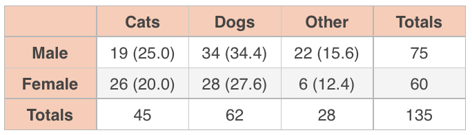
If you’ve done this correctly, the expected values should still sum to the same row and column totals.
The ???\chi^2??? distribution and degrees of freedom
This is where the ???\chi^2??? part comes in. We use the ???\chi^2??? formula to compare the actual and expected value in each cell, and then we sum all those values together to get ???\chi^2???.
???\chi^2=\sum\frac{(\text{observed}-\text{expected})^2}{\text{expected}}???
???\chi^2=\frac{(19-25.0)^2}{25}+\frac{(34-34.4)^2}{34.4}+\frac{(22-15.6)^2}{15.6}???
???+\frac{(26-20.0)^2}{20.0}+\frac{(28-27.6)^2}{27.6}+\frac{(6-12.4)^2}{12.4}???
???\chi^2=1.44+0.00+2.63+1.80+0.01+3.30???
???\chi^2=9.18???
In general, the larger the value of ???\chi^2???, the more likely it is that the variables affect each other (not homogeneous).
But to determine whether or not we can reject the null hypothesis, we need to look up the ???\chi^2??? value and the degrees of freedom in the ???\chi^2???-table. Similar to the normal- and ???t???-distributions, ???\chi^2??? has its own probability distribution that looks like this:
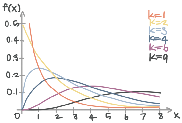
There’s a distinct ???\chi^2???-distribution for each degree of freedom. So you can see the ???\chi^2???-distribution for ???\text{df}=1??? in red, the ???\chi^2???-distribution for ???\text{df}=2??? in yellow, the ???\chi^2???-distribution for ???\text{df}=3??? in light blue, etc.
Of course, like the ???t???-table for ???t???-distributions, the ???\chi^2???-table for ???\chi^2???-distributions includes a degrees of freedom value.
The degrees of freedom is always the minimum number of data points you’d need to have all of the information in the table. So for example in a ???\chi^2???-test for homogeneity, degrees of freedom is given by
???\text{df}=(\text{number of rows}-1)(\text{number of columns}-1)???
When you calculate degrees of freedom, make sure you only include rows and columns from the body. Don’t include the total column or the total row. So for the table in the example we’ve been working with, we get
???\text{df}=(2-1)(3-1)???
???\text{df}=(1)(2)???
???\text{df}=2???
It makes sense that ???\text{df}=2??? for this example, because if we have any two pieces of information from the table, we can always figure out the rest of the information.
For instance, if we only know Male-Cats and Male-Dogs, we can find the rest of the missing values.

Taking Cats-Total minus Male-Cats gives Female-Cats; taking Dogs-Total minus Male-Dogs gives Female-Dogs; taking Male-Total minus Male-Cats minus Male-Dogs gives Male-Other, and then once we have Male-Other, taking Other-Total minus Male-Other gives Female-Other.
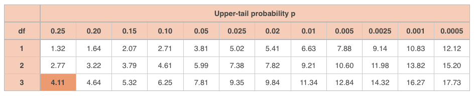
But back to the example, looking up ???\chi^2=9.18??? and ???\text{df}=2??? in the ???\chi^2???-table,

puts us between a ???p???-level of ???0.02??? and ???0.01???, closer to ???0.01???. So we could have picked an alpha value as high as ???\alpha=0.02??? and still rejected the null hypothesis, concluding that we’ve found support for the alternative hypothesis that gender affects pet preference (or that pet preference is affected by gender). But if we had picked an alpha value of ???\alpha=0.01???, we’d be unable to reject the null hypothesis.
So for this particular example, we can reject the null hypothesis and conclude that there’s a relationship between gender and pet preference (at ???\alpha=0.02???).
???\chi^2???-test for association/independence
In a ???\chi^2???-test for association or independence, we’re sampling from one group (instead of from two, like we did with the homogeneity test), but we’re thinking about two different variables for that same group.
In the example that follows, we’re taking a sample of employees at our company (sampling from one group), and looking at their eye color and handedness (two variables about them), so see whether or not eye color and handedness are associated.
Using a chi-square test

Take the course
Want to learn more about Probability & Statistics? I have a step-by-step course for that. :)
How to use a chi-square test for independence
Example
You want to know whether eye color and handedness are associated in employees of your ???15,000???-person company, so you take a random sample of company employees and ask them their eye color, and whether they’re left- or right-handed.
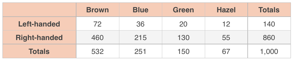
Use a ???\chi^2???-test for independence with ???\alpha=0.05??? to say whether or not eye color and handedness are associated.
Start by computing expected values.
Expected Left-Brown: ???(140\cdot532)/1,000=74.48???
Expected Left-Blue: ???(140\cdot251)/1,000=35.14???
Expected Left-Green: ???(140\cdot150)/1,000=21.00???
Expected Left-Hazel: ???(140\cdot67)/1,000=9.38???
Expected Right-Brown: ???(860\cdot532)/1,000=457.52???
Expected Right-Blue: ???(860\cdot251)/1,000=215.86???
Expected Right-Green: ???(860\cdot150)/1,000=129.00???
Expected Right-Hazel: ???(860\cdot67)/1,000=57.62???
Then fill in the table.
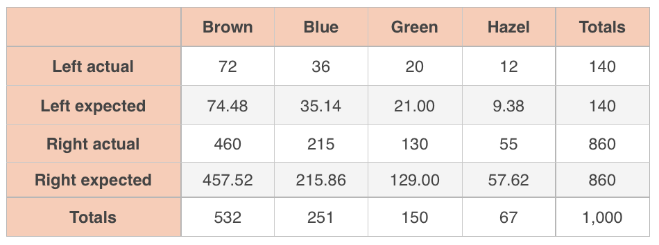
Now we’ll check our sampling conditions. The problem told us that we took a random sample, and all of our expected values are at least ???5??? (Left-Hazel has the smallest expected value at ???9.38???), so we’ve met the random sampling and large counts conditions. And even though we’re sampling without replacement, there are ???15,000??? employees in our company and we’re sampling less than ???10\%??? of them (???1,000??? is less than ???10\%??? of ???15,000???), so we’ve met the independence condition as well.
We’ll state the null hypothesis.
???H_0???: eye color and handedness are independent (not associated)
???H_a???: eye color and handedness aren’t independent (they’re associated)
Calculate ???\chi^2???.
???\chi^2=\frac{(72-74.48)^2}{74.48}+\frac{(36-35.14)^2}{35.14}+\frac{(20-21.00)^2}{21.00}+\frac{(12-9.38)^2}{9.38}???
???+\frac{(460-457.52)^2}{457.52}+\frac{(215-215.86)^2}{215.86}+\frac{(130-129.00)^2}{129.00}+\frac{(55-57.62)^2}{57.62}???
???\chi^2=0.082578+0.021047+0.047619+0.731812???
???+0.013443+0.003426+0.007752+0.119132???
???\chi^2\approx1.03???
The degrees of freedom are
???\text{df}=(\text{number of rows}-1)(\text{number of columns}-1)???
???\text{df}=(2-1)(4-1)???
???\text{df}=(1)(3)???
???\text{df}=3???
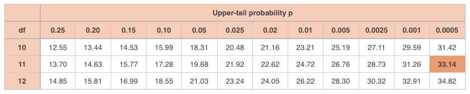
With ???\text{df}=3??? and ???\chi^2\approx1.03???, the ???\chi^2???-table gives
We’re off the chart on the left, which means we will definitely not exceed the alpha level ???\alpha=0.05???. Therefore, we fail to reject the null hypothesis, which means we can’t see an association between eye color and handedness, and we therefore assume that those two variables are not associated, which means they’re independent.

When we use a chi-square test for homogeneity, we’re trying to determine whether the distributions for two variables are similar, or whether they differ from each other.
???\chi^2???-test with contingency tables
In a ???\chi^2???-test for homogeneity, we sample from two different groups and compare whether their probability distributions are similar, and in a ???\chi^2???-test for independence, we sample from one group and try to determine the association between two variables about this one group.
But in a ???\chi^2???-test with a contingency table, we have a data table that gives some value or values, contingent upon some other condition.
For instance, in the example that follows, we’re working with a contingency table where we’re given cupcake sales by month. Which means we’re looking at cupcake sales, contingent upon the month of the year.
We’re not sampling from two different groups so it doesn’t make sense to use a ???\chi^2???-test for homogeneity, and we’re not sampling from one group to look at the relationship between multiple variables of theirs, so it doesn’t make sense to use a ???\chi^2???-test for association, either.
Instead, we’ll use a ???\chi^2???-test for a contingency table.
Example
A small cupcake company wants to know if their sales are affected by month. They’ve recorded actual sales over the past year and collected the data in a table. Use a ???\chi^2???-test with ???\alpha=0.05??? to say whether the company’s cupcake sales are affected by month.

The null hypothesis would be that sales aren’t affected by month.
???H_0???: sales aren’t affected by month (the month doesn’t affect sales)
???H_a???: sales are affected by month (the month does affect sales)
If sales aren’t affected by month, then they should be evenly distributed over each month, which means sales each month should be
???\text{expected monthly sales}=\frac{1,020\text{ total sales}}{12\text{ months}}=85\text{ sales per month}???
Which means we can expand the table to show actual versus expected sales.

Now that we have actual and expected values, we can calculate ???\chi^2???.
???\chi^2=\frac{(60-85)^2}{85}+\frac{(80-85)^2}{85}+\frac{(65-85)^2}{85}+\frac{(70-85)^2}{85}???
???+\frac{(80-85)^2}{85}+\frac{(100-85)^2}{85}+\frac{(140-85)^2}{85}+\frac{(120-85)^2}{85}???
???+\frac{(90-85)^2}{85}+\frac{(90-85)^2}{85}+\frac{(60-85)^2}{85}+\frac{(65-85)^2}{85}???
???\chi^2=\frac{625}{85}+\frac{25}{85}+\frac{400}{85}+\frac{225}{85}???
???+\frac{25}{85}+\frac{225}{85}+\frac{3,025}{85}+\frac{1,225}{85}???
???+\frac{225}{85}+\frac{225}{85}+\frac{625}{85}+\frac{400}{85}???
???\chi^2=\frac{7,250}{85}\approx85.29???
In a problem like this one, degrees of freedom is simply given by ???n-1???. Because looking at the body of the table, there are ???12??? pieces of information in the body (one for each month), and we would need ???11??? of these values in order to be able to figure out the ???12???th. So we can only be missing one pieces of data, and degrees of freedom is therefore ???n-1=12-1=11???. Look up ???\chi^2=\approx85.29??? and ???\text{df}=11??? in the ???\chi^2???-table.
With ???\text{df}=11???, the ???\chi^2??? value we found is off the chart. That’s telling us that there’s a massive difference between actual and expected values, which tells us that cupcake sales are very likely affected by month of the year. Which means we can reject the null hypothesis that sales aren’t affected by month of the year, and conclude that cupcake sales are affected by month.
Let’s walk through another example with a contingency table that looks a little different.
Example
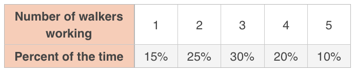
Marla owns a dog walking service in which she employees ???5??? of her friends as dog-walkers. She created a table to record the number of friends she believes are walking dogs for her at any given time.
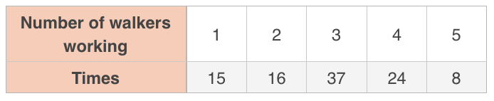
To test her belief, she took a random sample of ???100??? times and recorded the number of dog walkers working at that time.
Say whether a ???\chi^2???-test can be used to say whether her findings disagree with her belief. If a ???\chi^2???-test is valid, say whether her findings support her belief with ???95\%??? confidence.
Since Marla is sampling, we need to meet three conditions if she’s going to use a ???\chi^2???-test.
First, the sample needs to be random, and we were told in the problem that she took a random sample.
Second, every expected value needs to be at least ???5???. To find the expected values, we multiply her expected percentages by the total number of samples, ???100???.
The smallest of these expected values is ???10???, which is greater than ???5???, so we’ve met the large counts condition.
Third, Marla isn’t sampling with replacement, so the sample can’t be more than ???10\%??? of the total population. It’s safe to assume that Marla could continue taking an infinite number of samples at any given time, in theory gathering hundreds or thousands of samples as her business continues, so ???100??? samples shouldn’t violate the independence condition.
Therefore, it’s appropriate for her to use a ???\chi^2???-test. She’ll state the null hypothesis that her model for the number of friends walking dogs at any given time is correct (her model matches the actual counts that she collected).
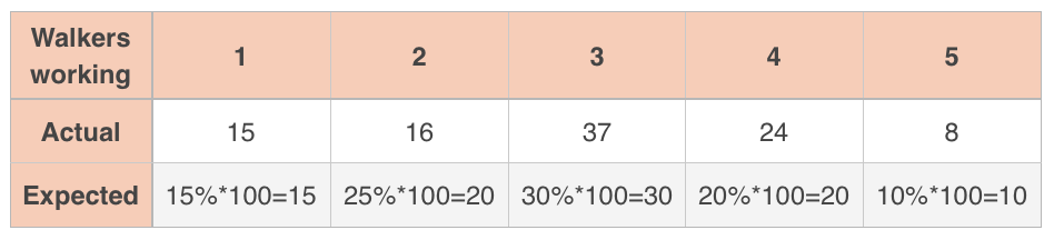
To compute ???\chi^2???, she’ll use the actual and expected values.
???\chi^2=\frac{(15-15)^2}{15}+\frac{(16-20)^2}{20}+\frac{(37-30)^2}{30}+\frac{(24-20)^2}{20}+\frac{(8-10)^2}{10}???
???\chi^2=\frac{0}{15}+\frac{16}{20}+\frac{49}{30}+\frac{16}{20}+\frac{4}{10}???
???\chi^2=\frac{109}{30}\approx3.63???
With ???5??? possibilities for number of walkers, there are ???4??? degrees of freedom, so look up ???\text{df}=4??? with ???\chi^2\approx3.63???.
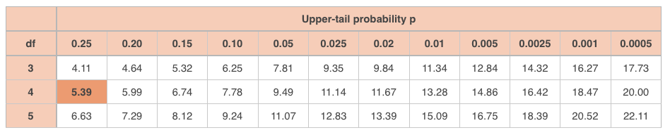
The value ???\chi^2\approx3.63??? is off the chart at ???\text{df}=4???. In order for Marla to reject the null hypothesis at ???95\%??? confidence, she would have needed to surpass a value of ???9.49??? to be above the ???5\%??? threshold.

Therefore, Marla cannot reject the null hypothesis, and can’t conclude that her model is correct. So she may want to consider adjusting her model to something that’s more in line with the data she collected, then collecting a new sample of data, and re-running the test to see if the new model seems to be more accurate.